Population Attributable Fractions¶

Population Attributable Fraction (PAF)

Population Attributable Fraction (PAF)¶

Measures of population impact estimate the expected health impact on a population if the distribution of risk factors that cause disease in that population is changed or removed. In GBD, this means lowering the level of exposure to disease causing risk factors to that of the theoretical minimum risk exposure level (TMREL, see TMREL section). Measures of impact take into account both the strength of the association (estimated by a measure of effect, like the rate ratio) and the distribution of the risk factor in the population. Measures of impact assume that we have established that the association between disease and risk factor is causal. If this assumption is true, population impact estimates measure how much of the disease in the population is caused by the suspected risk factor.

The population attributable fraction (PAF) is a measure of population impact. Intuitively, PAF equals (O − E)/O, where O and E refer to the observed number of cases and the expected number of cases under no exposure or a minimum exposure level, respectively. As an example, in early 1950, using the Doll and Hill case-control study of smoking and lung cancer deaths throughout England and Wales, Doll derived O = 11189 (observed number of cases in a population distributed with smokers and non-smokers) and E = 1875 (expected number of cases in a population of non-smokers). Therefore the smoking PAF for lung cancer deaths was (11189 − 1875)/11189= 83%; interpreted as 83% of lung cancer deaths was caused by smoking and if no one smoked, 83% of lung cancer cases can be avoided. The term “attributable” has a causal interpretation: PAF is the estimated fraction of all cases that would not have occurred if there had been no exposure (or TMREL level of exposure).

It is important to remember that measures of population impact are specific to the population studied, and can only be generalised to populations with exactly the same distribution of risk factors. Also note that risk factors that are strongly associations but which are rare, like being exposed to an X-ray in pregnancy and leukaemia in childhood, may have a large measure of effect but small measure of impact.

There are two main measures of population impact: 1) population attributable risk (PAR) and 2) population attributable risk fraction (PAF).

Population attributable risk (PAR)¶

Example 2x2 risk table:

	Exposed	Unexposed \| Total
With disease	a	c	a+c
Without disease	b	d	b+d
Total	a+b	c+d	a+b+d+c
Risk	r1 = a/(a+b)	r0 = c/(c+d)	r = (a+c)/(a+b+c+d)

The PAR is the absolute difference between the risk/rate in the whole population (r) and the risk/rate in the unexposed group (r0).

Population attributable risk (PAR) is calculated as

PAR = r - r0 Relative risk RR = r1/r0

Note that the risk difference (RD) in the earlier section contrasts the rate/risk in the exposed group (r1) and the rate/risk in the unexposed group (r0 = r1-r0).

If we know the risks among the exposed (r1) and unexposed (r0), and the prevalence of exposure in the population ( \(p_p\) )

\[PAR = p_p (r1-r0)\]

where

\[p_p = \frac{a+b}{a+b+c+d}\]

The prevalence of exposure in the population is

It can be shown that

PAR = r - r0
    = (a+c)/(a+b+c+d) - c/(c+d)
    = (ad-bc)/[(a+b+c+d)(c+d)]

PAR =  .. math:: p_p (r1-r0)
    = (a+b)/(a+b+c+d) x [(a/(a+b) - c/(c+d)]
    = (ad-bc)/[(a+b+c+d)(c+d)]

Population attributable risk fraction (PAF)¶

The population attributable fraction is a quantification of the proportion of a given cause outcome, such as cases, deaths, or DALYs, that could be eliminated by removing a risk exposure. It is the proportion of all cases in the whole study population (exposed and unexposed) that may be attributed to the exposure, assuming a causal association. The population attributable risk fraction (PAF) is estimated by dividing the population attributable risk by the risk in the total population (r).

PAF = PAR/r

= (r - r0) / r

When only the risk ratio (RR) and the prevalence of exposure in the population are known, PAF can also be written as:

\[\text{PAF}=\frac{p_p(RR-1)}{1+p_p(RR-1)} ...(a)\]

Note that the PAF increases with the rate ratio θ, but also with the prevalence of exposure p. It will therefore vary between populations, depending on how common the exposure is.

It is important to note the PAF in equation (a) will give us an accurate representation of the porportion of cases occuring in the total population that would be avoided if the exposure were removed only if the assumptions that 1) the observed association between exposure and disease is causal, and that 2) it is free from confounding and bias.

Todo

I’m wondering if it is it possible to illustrate this using DAGs? or visually? I’ll have a think

Although equation (a) is the best-known formula for the PAF and the one used in GBD PAF calculations, there is an alternative formulation which can be useful when we wish to take account of confounders and joint effects

If you know the prevalence of exposure among cases (\(p_c\)) there is a very useful formula for PAF which can be used with risk or rate ratios that have been adjusted for confounding:

\[\text{PAF}=\frac{p_c(RR_{adj}-1)}{RR_{adj}} ...(b)\]

The following diagram illustrates how the PAF is derived intuitively from the prevalence of exposure among cases (\(p_c\))

../../../../_images/PAF_intuitive_diagram.svg

However, it is not always possible to find the prevalence of exposure among cases (\(p_c\)) and so equation (a) is used in our simulation models. This will introduce bias. The following section talks about the bias that occurs.

Bias in PAF Calculation ¶

The PAF can be calculated using the following formula:

(1)¶\[\text{PAF}=\frac{p_c(RR_{adj}-1)}{RR_{adj}}\]

In which we define \(p_c\) to be the proportion of cases (individuals who possess the outcome of interest) that are exposed, and \(RR_{adj}\) has been adjusted for confounding and effect modification.

There is the a second PAF equation, which can be used in the absence of confounding or effect modification:

(2)¶\[\text{PAF}=\frac{p_p(RR_{cr}-1)}{1+p_p(RR_{cr}-1)} =\frac{p_p(RR_{adj}-1)}{1+p_p(RR_{adj}-1)}\]

Note that here, the crude relative risk \((RR_{cr})\) is equivalent to the adjusted \((RR_{adj})\). We define \(p_p\) to be the proportion of the entire population that is exposed.

This is typically easier to conceptualize if we break the population down as follows:

Exposure x Cases¶
	Cases	Non-cases
Exposed	a	b
Unexposed	c	d

Observe that the above table is a full partition of our population. We can see then that the proportion of cases that are exposed is given by:

\[p_c=\frac{a}{a+c}\]

And the proportion of the entire population that is exposed is given by:

\[p_p = \frac{a+b}{a+b+c+d}\]

It can be shown that when the fraction of cases in the unexposed times the relative risk \(\left( \frac{c}{c+d} \cdot RR_{adj} \right)\) equals the fraction of cases in the exposed \(\left( \frac{a}{a+b} \right)\), i.e., when there are no confounders or effect modifiers, equation (1) equals equation (2).

However, when \(\frac{c}{c+d} \cdot RR_{adj} \neq \frac{a}{a+b}\), equation (1) does not equal equation (2). Intuitively, we can imagine a confounder that is positively associated with our exposure, holding all else constant. Then there will be a disproportionately high number of cases among the exposed, and \(\frac{c}{c+d} \cdot RR_{adj} < \frac{a}{a+b}\).

This can be solved via weighting equation (2) per stratum of our confounder or effect modifier, yielding equation (3):

(3)¶\[\text{PAF} = \sum_{i=1}^z W_i \frac{p_i(RR_i-1)}{1+p_i(RR_i-1)}\]

Here, for each stratum \(i\) of our confounder or effect modifier, \(p_i\) is the proportion of the stratum that is exposed, \(W_i\) is the proportion of the cases in the stratum, and \(RR_i\) is the stratum-specific adjusted RR. Note that in the case of a confounder, \(RR_{i}\) will be equal across strata, and in the case of effect modification, there will be a different \(RR_{i}\) per stratum. More information on confounding and effect modification can be found in the section on causal relationships.

While we know equation (2) to be biased, we have had to use it in Vivarium modeling due to insufficient data for use of equation (2) or (3).

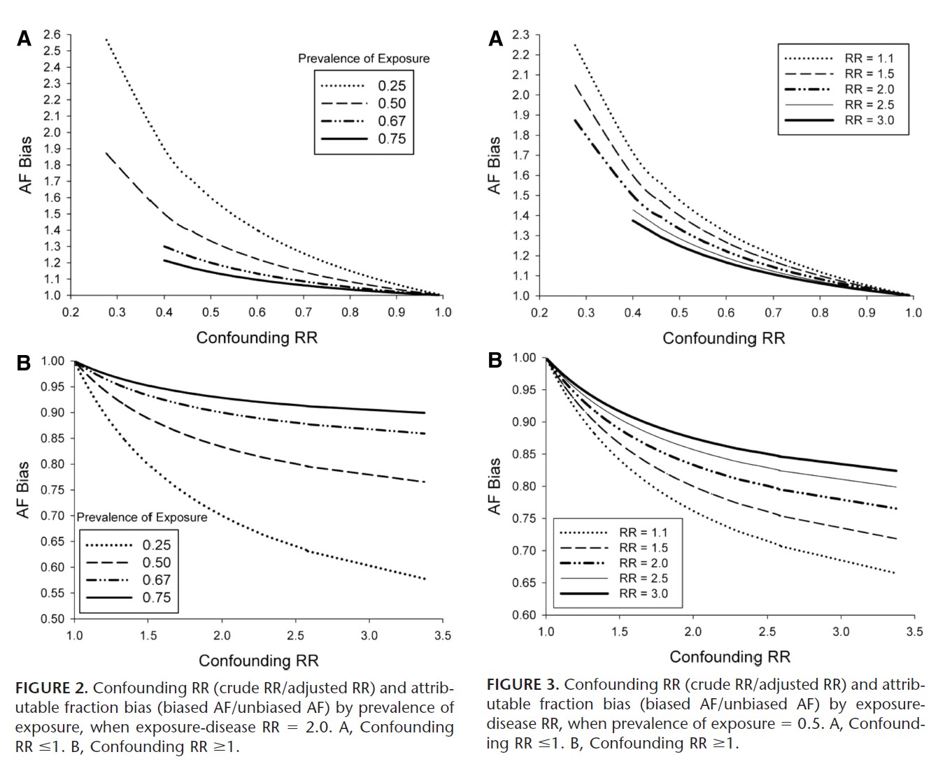
The following is a high-level summary of a the paper Confounding and Bias in the Attributable Fraction by [Darrow], which examines the direction and magnitude of this bias for different scenarios. This was achieved by generating synthetic data with varying degrees of exposure prevalence, confounding, relative risk for the disease (or cause), and prevalence of the confounder in the exposed and unexposed groups. These scenarios were all examined for one dichotomous confounder; however, Darrow then showed these results generalize to two dichotomous confounders.

We consider PAF bias primarily in terms of the following ratio:

\[\frac{\text{biased PAF}}{\text{unbiased PAF}}\]

Where the biased PAF is calculated using equation (2), and the unbiased PAF is calculated using equation (3).

Direction ¶

The direction of this bias was found to be fully determined by the confounding risk ratio:

\[\frac{RR_{crude}}{RR_{adj}}\]

Here, \(RR_{adj}\) is the Mantel-Haensel adjusted RR. A positive counfouding RR (\(>1.0\)) resulted in a negative PAF bias, and a negative confounding RR (\(<1.0\)) resulted in a positive PAF bias.

Furthermore, the direction of the confounding RR is fully determined by (1) the direction of the association between the confounder and the exposure, and (2) the direction of the association between the confounder and disease (or cause).

This relationship is captured as follows:

Direction of Bias in the PAF¶
Confounder-exp n assoc.	Confounder-cond’n assoc.	Confouding ratio	PAF bias
\(+\)	\(+\)	\(>1.0\) \((+)\)	\(-\)
\(-\)	\(-\)	\(>1.0\) \((+)\)	\(-\)
\(-\)	\(+\)	\(<1.0\) \((-)\)	\(+\)
\(+\)	\(-\)	\(<1.0\) \((-)\)	\(+\)

Magnitude ¶

The magnitude of the PAF bias was shown to increase with:

lower exposure prevalence

smaller \(RR_{adj}\) for the disease (or cause)

magnitude of the confounding RR

The first two factors are intuitive: observe that in our measure of bias, \(\frac{\text{biased PAF}}{\text{unbiased PAF}}\), a smaller exposure prevalence will lead to a smaller true PAF in the denominator, amplifying the bias. Similarly, a smaller \(RR_{adj}\) will also result in a smaller true PAF, again amplifing the bias.

However, when examining the absolute difference between the biased and unbiased PAFs, note that Darrow did not find that lower exposure prevalence necessarily caused a larger absolute PAF bias.

For the confounding RR, we note that by “magnitude” we mean distance from confounding RR =1. That is, as a confouding RR <1 decreases, it causes an increased overestimation of the PAF, and as a confounding RR>1 increases, it causes an increased underestimation of the PAF.

Darrow states that the amount of bias under most realistic scenarios is on the order of 10%-20%. Note that this percentage describes the percentage difference between the biased and unbiased PAF. That is, if the true PAF is 50%, and the biased PAF is 40%, we characterize this as a 20% negative bias.

Below we include graphs from the paper illustrating PAF bias as a function of exposure prevalence and RR.

Other sources of bias ¶

Darrow concludes by noting that the PAF is highly sensitive to the relative risk, exposure prevalence, and distribution of confounders. Thus when relative risk and exposure prevalence data is collected from published papers, if one tries to apply these measures to a target population with different population characteristics and without sufficient data to correctly calculate the PAF, the bias caused by the differing distributions between the study and target populations can result in vastly more bias than that of using the wrong PAF equation.

Estimation of the PAF in epidemiological studies ¶

Todo

detail this section more and give modified PAF for each study design

Cohort studies: Simplest situation, since disease rates in exposed and unexposed can be measured directly Cross-sectional studies: Prevalence of a disease state is measured, rather than its incidence. Unmatched case-control studies: Ratio of two proportions, given independent samples Matched case-control studies: Can use alternative equation in this case, providing the cases can be regarded as a representative sample of all cases. Exposure with multiple levels: Estimate the proportion of cases attributable to each level of exposure, the proportion of cases that would be avoided if the rate of disease in each exposure group were reduced to that in the unexposed (or baseline) group. There are some caveats to the cohort studies estimation of PAF, if exposed and unexposed cohorts have been sampled separately for the study. A separate estimate of p or p’ will be required.

In cross-sectional studies, this is also known as the proportion of prevalent cases in the population. There are some potential issues this type of study of interpreting prevalence rather than incidence cases. If an exposure is associated with increased prevalence of disease, it could be because the exposure increases the risk of developing the disease, or because it increases the amount of time a person has the disease, or even because it increases survival from the disease.

This use of PAF is recommended for chronic disease states.

References ¶

Darrow: Confounding and bias in the attributable fraction, Jan 2011 https://www.ncbi.nlm.nih.gov/pubmed/20975564