Causes

What is included in this chapter: models of causes that are represented as finite-state Markov chains (this chapter will also explain what a finite state Markov chain is!)

There are models of things that you might consider causes which are outside of the scope of this chapter, because they do not fit into the Markov approach. This chapter does not include PAF of 1 causes, like protein energy malnutrition. It also does not include things that are sometimes considered diseases but are deemed risk factors by the Global Burden of Disease (GBD), such as obesity. Unsafe water would not fit into the cause model paradigm either—it is a cause of diarrheal disease, but it is a risk factor in the GBD taxonomy. Latent tuberculosis infection (LTBI) does fit into this chapter, but just barely. Impairments have additional, targeted information on a separate page. If you’re not sure what an impairment is or how it might be different than a cause, check out this :ref: page explaining causes, impairments, and related GBD terms. <GBD_disease_health>

What is a “cause” and what is a cause model?

When we say “cause” in simulation modeling with vivarium, we often mean a disease.

There is a reason for this potentially confusing terminology: a “cause of death”, as might be included as the bottom line of the top half of a death certificate, is often a disease but sometimes an injury. And we extend this to also refer to causes of nonfatal health loss, too.

A cause model is a simplification of a cause of death or disease for the purposes of simulation modeling. It is always an idealization of the messy complexity of reality, and is designed to be acceptable to outside experts on the cause, as well as be parsimonious with the data available from the GBD that might inform the model.

Todo

Link to GBD hierarchies for production of YLLs and YLDs. Add discussion of the discrepancy between our cause models (unified dynamic models of prevalence, incidence, mortality & morbidity) and GBD models (separate statistical models of mortality & morbidity only, with intermediate (e.g. dismod) unified models). Note where this might cause modeling issues!

Might be better as a separate section.

Learning objectives

After reading this chapter, learners should be able to:

1. Develop an understanding of how the GBD, literature, and experts think about a cause. [[to come]]

2. Build internally consistent cause models which are sufficiently complex given larger modeling goals. [[to come]]

   1. Models that are as simple as possible, but no simpler.

   2. Models that agree with withheld data.

   3. Models that captures the outcomes of interest. (Which is really the same as “but no simpler” in (a))

3. Document the models in a way software engineers can build and verify it, and document their understanding comprehensively for future researchers (including their future selves) who are faced with related modeling challenges.

How is a cause model incorporated into a larger model?

Our modular structure is designed to layer cause models into the entity component system that has a demographic model. Sometimes an intervention model will be layered in on top of this and directly change transition rates in one or more cause models. But to date, it has been more common to have one or more risk factor models layered in to affect the incidence rates in the cause model, and then have an intervention model shift the risk exposure levels defined by the risk factor model.

It can be useful to consider two separate ways that a cause models fits into a larger model: (1) how does a cause model affect other parts of the model? and (2) how is a cause model affected by other parts of the model?

[[More details on this to come]]

Why do we want a document that describes each cause model?

• Because a lot of work goes into gaining understanding and developing an appropriately complex model, and we don’t want to repeat that work.

• Because we (researchers) need to communicate clearly and precisely with software engineers, data scientists, and each other about what the model must do and what data must inform it.

• Because we will need to communicate to an outside audience, including critics, how we generated substantive results of interest, and that will include readers who want to know exactly how we modeled the diseases included in our work.

What does a model document look like?

• Title which is descriptive

• Cause model diagram

  • Set of states that are “mutually exclusive and collectively exhaustive”—a single agent is in exactly one of these states at any point in time.

  • Set of transitions between states.

• Definition of model and states.

• Restrictions: who does this apply to?

• How to initialize the states? (prevalence data)

• Definition of transitions in terms of states they connect.

• Transition criteria (rates, durations, deterministic, etc.)

• How does this model connect to other models. That is, what outcomes this disease influences? (e.g. disability, mortality, or incidence)

• What data informs those connections?

• “Theory of disease” meaning is this a “susceptible-infected” model (SI), is a recurrent MI model, etc? This prose should match and complement the cause model diagram.

• Validation criteria

• Assumptions about the model

[[to be updated based on experience from LTBI cause model document, and generalization thereof]]

Basic Cause Model Structures

Todo

Link to examples of cause model documents

Common basic cause model structures are described in the following table and dicussed in further detail below. Notably, cause models are almost always more complicated than the basic structures discussed in this section. The following basic structures should be considered as basic guiding concepts, and not as templates that are appropriate for all (or even most) cause models. Examples of more complicated cause model structures are discussed in the Other Cause Model Structures section afterward.

Basic Cause Model Structures

Model	States	Description
SI	Susceptible-Infected	Simulants never recover from the infected (with condition) state
SIS	Susceiptible-Infected-Susceptible	Simulants can recover from the infected (with condition) state and can become infected again after recovery
SIR	Susceptible-Infected-Recovered	Simulants can recover from the infected (with condition) state and cannot become infected after recovery

SI

In this cause model structure, simulants in the susceptible state can transition to the infected state, where they will remain for the remainder of the simulation.

This cause model structure is appropriate for chronic conditions from which individuals can never recover.

Examples of conditions potentially appropriate for an SI cause model structure include Alzheimer’s disease and other dementias.

SIS

In this cause model structure, simulants in the susceptible state can transition to the infected state and simulants in the infected state can transition to the susceptible state. Notably, this cause model allows for simulants to enter the infected state more than once in a simulation.

This cause model structure is appropriate for conditions for which individuals can have multiple cases over their lifetimes.

Examples of conditions potentially appropriate for an SIS cause model structure include diarrheal diseases.

SIR

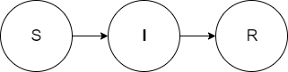
In this cause model structure, simulants in the susceptible state can transition to the infected state and simulants in the infected state can transition to a recovered state where they will remain for the remainder of the simulation. Notably, the cause model allows individuals to become infected only once in a simulation.

This cause model structure is appropriate for conditions for which individuals can only have a single case, but do not stay in the with condition state forever.

An example of a condition potentially appropriate for an SIR cause model structure is measles.

Other Cause Model Structures

It is common that a particular cause may not fit well into one of the common basic cause model structures discussed above. Examples of situations that may require custom cause model structures are listed below:

• Cause models with severity splits

• Joint cause models (multiple closely related causes represented in a single cause model)

• Neonatal/Congenital cause models

• Other scenarios required by the specifics of a given cause

Data Sources for Cause Models

Once a cause model structure is specified, data is needed to inform its states and transitions. For our purposes, cause models generally have the following data needs:

Cause Model Initialization

Which cause model state will a simulant begin the simulation in?

Cause Model Transitions

How and when does a simulant move between cause model states?

Mortality Impacts

How and when does a simulant die and how does this differ depending on the specific cause model state that the simulant occupies?

Morbidity Impacts

How does a simulant experience morbidity and how does this differ depending on the specific cause model state that the simulant occupies?

Restrictions

For which population groups (e.g. age and sex groups) is this cause model not valid?

Our cause models use approximately instantaneous, individual-based probabilities to make decisions about how an individual simulant moves about a cause model. Because we cannot possibly predict the exact moment a specific individual will get sick or die, we use population-level estimates as our best-guess predictors for individual-level estimates.

For instance, we don’t know if Jane Doe will die in the next year, however, we can use information on the overall rate of death in Jane Doe’s population to make a guess on the probability that Jane Doe will die in the next year.

We can increase the quality of this guess by adding detail to the model we use to make our guesses. For instance, if we know Jane Doe has HIV, we can use the rate of death among individuals with HIV to make a better guess at the probability Jane Doe will die in the next year.

There are several common population-level data sources that are used to inform our cause models. These data sources are outlined in the table below and discussed in more detail afterward.

Data Definitions

Measure	Definition	Model Application	Specific Use
Prevalence	Proportion of population with a given condition.	Initialization	Represents the probability that a simulant will begin the simulation in a with-condition cause model state.
Birth Prevalence	Proportion of all live births born with a given condition.	Initialization	Represents the probability that a simulant born during the simulation will be born into a with-condition cause model state.
Incidence Rates	Number of new cases of a given condition per person-year of the at-risk population.	Transition rates	Once scaled to simulation time-step, represents the probability a simulant will transition from infected to recovered.
Remission Rates	Number of recovered cases from a given condition per person-year of the population with the condition.	Transition rates	Once scaled to simulation time-step, represents the probability a simulant will recover from the with-condition state.
Duration	Length of time a condition lasts.	Transition rates	Amount of time a simulant remains in a given state
Progression	Transition from a lower severity state to a higher severity state within a given cause model.	Transition rates	Used to determine prevalence of a given condition by severity.
Severity Splits	Separation of a cause into different states by severity.	Transition rates	Used to determine prevalence of a given condition by severity.
Restrictions	List of groups that are not included in a cause.	General	List of population groups for which the cause model does and does not apply.
Disability Weights	Proportion of full health not experienced due to disability associated with a given condition.	Morbidity impacts	Rate at which an individual accrues years lived with disability due to the state in the cause model.
Cause-specific Mortality	Measure of deaths due to a particular cause per person-year in the overall age-, sex-, time-, and location-specific population.	Mortality impacts	Used to determine a simulant’s mortality hazard rate.
Excess Mortality	Measure of deaths due to a particular condition per person-year in the age-, sex-, time-, and location-specific population with that condition.	Mortality impacts	Used to determine a simulant’s mortality hazard rate.

Cause Model Initialization

Prevalence

Prevalence is defined as the proportion of a given population that possesses a specific condition or trait at a given time-point.

For example, the prevalence of diabetes mellitus in the United States was approximately 6.5% in 2017.

Notably, GBD prevalence estimates for a given year (e.g. 2017) are meant to represent the point prevalence at the midpoint of that year (e.g. 7/1/17).

Prevalence data can be used to initialize cause model states and represents the probability that a simulant will begin the simulation in a given state.

For example, the probability that a simulant in a model of diabetes mellitus in the United States beginning in 2017 will begin the simulation with diabetes is 0.065, or 6.5%.

Notably, prevalence is used to initialize cause model states in the following scenarios:

• A simulant enters the simulation at the start of the simulation

• A simulant enters the simulation due to immigration to the simulated location

• A simulant enters the simulation by aging into the simulation

  Prevalence is not used to initialize cause model states when a simulant is born into a simulation. See the below section on birth prevalence for how cause model states are initialized in this scenario.

GBD results of cause prevalence are estimates of point prevalence at the year midpoint. Notably, Vivarium assumes that the prevalence of a given cause is constant across the entire year that it represents. This is likely an appropriate assumption in cases where prevalence is relatively constant over time and over age groups, although it may be limited in cases where it is not.

Birth Prevalence

Birth prevalence is defined as the proportion of live births in a given population that possess a given condition or trait at birth.

For example, the birth prevalence for cleft lip in the United States in 2006 was 10.6 per 10,000 live births, or 0.106%.

Birth prevalence data can be used to initialize neonatal cause model states and represent the probability that a simulant who is born during the simulation will be born into a given neonatal cause model state.

For example, the probability that a simulant born during a simulation of cleft lip in the United States in 2006 is 0.00106, or 0.106%.

Cause Model Transitions

Todo

Enhance blurb to beginning of cause model transition section about how we use probabilies to inform cause model transitions (to come in next commits)

Limitations/assumptions of incidence rates section

Detail remaining transition rate data sources (remission, duration, severity splits, deterministic)

Vivarium uses probabilities to make decisions about how and when simulants move between cause model states.

Incidence Rates

Generally, incidence is a measure of new cases of a given condition that occur in a specified timeframe and population. The count value of new cases of the condition of interest will always be the numerator of incidence measures. The denominator of incidence measures is somewhat more complex and is critical to ensuring an accurate data source to inform cause model transition rates.

Two incidence measures relevant to cause model transition rate data sources using GBD results are discussed in this section, including measures we refer to as incidence in the total population (as estimated by the GBD study) and incidence in the susceptible (or at-risk) population. These measures are defined using the following key concepts:

Person-time: person-time is a measure of the number of individuals multiplied by the amount of time they individually occupy the population of interest. Notably, the population of interest varies depending on context and can be defined by age group, sex, location, time, disease status, etc.

For example, if one individual is occupies the population of interest for two years, they contribute two person-years. If another individual is in our population of interest for 6 months, they contribute 0.5 person-years. Together, these two individuals contribute a total of 2.5 person-years.

Susceptible or At-Risk Population: the susceptible population, also referred to as the at-risk population, is defined as the population that * does not* have the condition of interest; in other words, the susceptible population that is at risk of developing the condition. Notably, the number of individuals in this population will change over time as the following events occur:

• Members of the at-risk population develop the condition and are no longer susceptible

• Members of the at-risk population die and are no longer susceptible

• Individuals are born or age into the at-risk population and become susceptible

• Individuals age out of the at-risk population and are no longer susceptible

• Individuals with the condition recover from the condition and re-enter the at-risk population as susceptible (in the case of conditions with remission)

Total Population Incidence Rate is estimated by the Global Burden of Disease Study by estimating the number of incident cases that occur in one year and scaling this value per 100,000 individuals of a specified population.

\[\frac{n_\text{incident cases}}{\text{person-time}_\text{total population}}\]

Because the denominator of this measure is not specific to a particular cause model state, it is not an appropriate data source for cause model transition rates between states.

Note

GBD estimates of total population incidence rate require transformation prior to use as a cause model transition probability data source (see below for more detail).

Susceptible/At-Risk Population Incidence Rate as discussed here is also referred to as incidence density rate, person-time incidence rate, and in some cases may simply be referred to as the incidence rate. It is defined as:

\[\frac{n_\text{incident cases}}{\text{person-time}_\text{susceptible population}}\]

Because the denominator for the susceptible population incidence rate is person-time in the at-risk population, this incidence rate can be used to compute the probability of a new case of the condition occuring in an individual without the condition in a given time frame. Therefore, it can be used to compute the probability that a simulant will transition from a susceptible to infected cause model state in a given timestep.

For instance, consider an example in which the global susceptible population incidence rate of injuries in 2017 was 6,800 cases per 100,000 person-years, or 0.068 cases per person-year. In this example, 6,800 new injuries occurred among 100,000 person-years of observation among the non-injured population.

Now, consider a cause model with a susceptible (not injured) state and an infected (injured) state with a simulation timestep of 1 year. In this case, the probability that a simulant will transition from the susceptible to infected state within a single timestep (i.e. the transition probability) would be represented as 0.068.

Notably, in order to represent the transition probability for a single simulant within a single timestep, the cumulative incidence value needs to be scaled so that the person-time denominator is equal to the simulation timestep. Therefore, if the timestep of the cause model considered above were six months instead of one year, the transition probability would be 0.034 (0.034 cases per 0.5 person-years).

Note

Because GBD estimates total population incidence rates, Vivarium automatically transforms GBD results into susceptible population incidence rates that can be used as an appropriate data source for cause model transition probabilities.

This transformation from total population incidence rate to an approximation of the susceptible population incidence rate is performed with the following calculation:

\[\frac{\text{Total Population Incidence Rate}}{(1-\text{Condition Prevalence})}\]

There are several key assumptions and limitations to the approach of using GBD incidence rates as data sources for cause model transition rates, disscussed below.

Todo

Add discussion of transformation of GBD estimates of total population to susceptible population incidence rates

Add discuission about assumption that transition probability is constant over time frame and link to hazard rates page for when this might be an issue. Include formulas about how we are approximating hazard rate.

Add discussion about how cause model transition probabilities are state-specific and not necessarily cause-specific. Cannot use cumulative incidence of disease to represent the transition probability from susceptible to moderate disease directly, for example. (maybe use LTBI as an example here)

Remission Rates

Definition

Remission is a measure of cases that recover from a with-condition state, given a specified population and time period. Just as with incidence, the numerator is given by the count of recovered (or remitted) cases, and the denominator is the cumulative person-time during which cases are able to go into remission:

\[\frac{\text{number of remitted cases}}{\text{person-time in the with-condition population}}\]

For example, consider diarrhea cases in the Philippines in 2017. Say that in the year under consideration, every such case remitted after an average of 5 days:

\[\frac{\text{1 case}}{\text{5 person-days}} = \frac{\text{1 case}}{\text{5 person-days}} \times \frac{\text{365 person-days}}{\text{1 person-year}}=\frac{73\text{ cases}}{\text{1 person-year}}\]

This calculation is straightfoward, as diarrheal diseases have a highly consistent disease duration.

In contrast, consider diabetes. Say that there were 142,794 prevalent cases of diabetes (both type I and type II) in Moldova amongst males in 2017, and of those 142,794 cases, 509 remitted in 2017. This gives us the following rate:

\[\frac{\text{509 cases}}{\text{142,794 person-years}} = \frac{\text{0.0036 cases}}{\text{1 person-year}}\]

It is important to note two things here: first, that this is a remission rate for diabetes at all ages, which obscures the generally increasing age-pattern that this rate follows. Second: there is no set duration for which one generally experiences diabetes. In fact, remission does not occur for type I, and is not guaranteed for type II. In the context of the diarrheal diseases example, this makes it seem as if diabetes cases remit, on average, after \(\frac{1}{0.0036}\simeq 279\) years–which clearly does a poor job of capturing the behavior of diabetes. This sort of description was only appropriate for diarrhea, as there is a uniform remission rate across all cases. With diabetes, however, the remission rate does not tell us the average duration that an individual will experience diabetes.

How do we apply this to our simulants? Say we randomly selected 10 people with diarrhea in the Philippines on a random day in 2017. In the next day, they would accumulate 10 person days. Our rate tells us that in the next day, the expected value for cases remitted is given by:

\[\frac{\text{1 case of diarrhea}}{\text{5 person-days}}\times\text{10 person-days} = \text{2 remitted cases of diarrhea}.\]

Similarly, we can take the rate of remission of diabetes, and for a randomly selected case of diabetes in Moldova in 2017, consider if they will remit some time in the next year. The expected value for cases remitted is then given by:

\[\frac{\text{0.0036 cases of diabetes}}{\text{1 person-year}}\times\text{1 person-year} = \text{0.0036 remitted cases of diabetes}.\]

Note that when we refer to remission rates, we are typically considering a rate within the infected or with-condition population. This is true both in general, and in the context of GBD–unlike with incidence, which GBD calculates within the entire population, as discussed above.

Remission within GBD

Most nonfatal models in GBD are run using DisMod (Cause Models). DisMod estimates compartmental models of disease, and thus produces estimates of measures (prevalence, incidence, remission, excess mortality rate, etc.) that are internally consistent for any given model. DisMod estimates remission rates as:

\[\frac{\text{number of remitted cases}}{\text{person-years in the with-condition population}}\]

Todo

update link to dismod page, once available

GBD’s final outputs, however, are in the form of YLLs, YLDs, and DALYs. To calculate these measures such that they are consistent across different causes, GBD runs standardizing processes on estimates of prevalence, incidence, and estimated mortality rate. Note then that these final estimates are no longer consistent with the DisMod estimates. However, as remission is not needed to calculate YLDs, the latest-stage estimate of remission produced by GBD comes from DisMod models.

Implementing remission rates in cause models

For a given simulation with timesteps of length time unit and a given time unit, we convert remission rates to the form of cases remitted per person-time-unit. If the rate is small with respect to the timestep (that is, if the rate is less than 1 per the time step), it can be used to compute the probability of a simulant transitioning from an infected or with-condition state to a susceptible or free-of-condition state in a given timestep.

Duration-Based Transitions

Deterministic or Triggered Transitions

Progression Transitions

Severity Splits

Mortality Impacts

All-Cause Mortality

All-cause mortality rate (ACMR) is a measure of total deaths (due to all causes) per person-year in the overall age-, sex-, time-, and location-specific population. Specifically,

\[\frac{\text{number of deaths due to all causes}}{\text{person-years in the overall population}}\]

For instance, the global ACMR for the early neonatal age group (0-6 days) in 2017 was approximately 70,000 deaths per 100,000 person-years (0.7 deaths per person-year). However, the global ACMR for the post neonatal age group (1 month to 1 year) in 2017 was approximately 1,000 deaths per 100,000 person-years (0.01 deaths per person-year). By comparing ACMRs between these age groups, we can see that individuals die at a higher rate during the early neonatal period than the post neonatal period.

Notably, ACMR is used both for validation of Vivarium simulations, as well as for estimating simulation mortality rates (see the Mortality Hazards section for more detail).

Cause-Specific Mortality

Cause-specific mortality rate (CSMR) is a measure of deaths due to a particular cause (or group of causes) per person-year in the overall age-, sex-, time-, and location-specific population. Specifically,

\[\frac{\text{number of deaths due to cause}}{\text{person-years in the overall population}}\]

For instance, the global CSMR for mesothelioma in 2017 was approximately 0.4 deaths per 100,000 person-years. The global CSMR for diabetes mellitus in 2017 was approximately 18 deaths per 100,000 person years. By comparing these two CSMRs, we can see that more individuals in the overall global popultaion died due to diabetes mellitus than mesothelioma in 2017.

Note

The concept of cause-specific mortality as we discuss here (and as it is used in the Global Burden of Disease study and Vivarium simulations) implies that there is always one single cause of death for an individual. This may be a reasonable assumption in some cases, for instance, death due to a traffic accident. However, ascertaining a single cause of death can be more complicated in other cases; imagine an individual is in a serious traffic accident and the stress of the accident causes them to have a heart attack – did the traffic accident or the heart attack cause the death of this individual?

If interested, see this publication by Piffaretti et al. (2016) that discusses the classical single cause of death analysis and proposes an alternative approach that weights multiple causes of death.

Notably, CSMRs are useful for validation of Vivarium simulations, as well as for estimating simulation mortality rates (see the Mortality Hazards section for more detail).

Excess Mortality

Excess mortality rates (EMRs) are a measure of the rate at which individuals with a given condition die due to that position; in other words, the number of deaths due to a particular condition per person-year in the age-, sex-, time-, and location-specific population with that condition. Specifically,

\[\frac{\text{number of deaths due to cause}}{\text{person-years spent infected with cause}}\]

Or, approximately,

\[\frac{\text{CSMR per 100,000 person years}}{\text{Prevalence of cause per 100,000}}\]

For instance, the excess mortality rate of mesothelioma in 2017 was approximately 0.38 while the excess mortality rate of diabetes mellitus was 0.003, indicating that mesothelioma is a more fatal disease than diabetes mellitus once acquired. Contrast this with the cause-specific mortality rates for these two conditions discussed above; mesothelioma has a higher EMR but lower CSMR than diabetes mellitus. This means that while someone with mesothelioma is more likely to die due to mesothelioma than someone with diabetes is to die due to diabetes because mesothelioma is more fatal (as reflected by the higher EMR), someone in the general population is less likely to die of mesothelioma than of diabetes because mesothelioma is much less prevalent than diabetes (as reflected by the lower CSMR).

Notably, EMRs are useful for validation of Vivarium simulations, as well as for estimating simulation mortality rates (see the Mortality Hazards section for more detail).

Note

The application of EMRs in Vivarium simulations allow for the consideration that an individual with a given cause is at an increased mortality rate for that cause. However, it does not necessarily allow for the consideration that an individual with that cause may also have an increased mortality rate for other causes due to the impact of comorbidities. While this phenomenon can be represented for some causes through the GBD risk factors framework (ex: vitamin A deficiency is related to increased mortality due to measles), our modeling framework is limited in that it does not consider the effect of comorbidities outside of GBD risk factors.

Mortality Hazards

At each time-step in a Vivarium simulation it must be determined if each simulant remains alive or dies. The probability that a simulant will die is assessed using the mortality hazard for an individual simulant, \(i\), as shown below:

In a simulation with only one cause, \(c\):

\[\text{mortality hazard}_i = ACMR - CSMR_c + C_i * EMR_c\]

Where,

• \(ACMR\) is the all-cause mortality rate specific to the simulant’s age, sex, time, and location group

• \(CSMR\) is the cause-specific mortaltiy rate for cause \(c\) specific to the simulant’s age, sex, time, and location group

• \(C_i\) is a variable that indicates the cause state for an individual simulant so that it is equal to 1 if a simulant is with condition \(c\) and equal to 0 if a simulant is without condition \(c\)

• \(EMR_c\) is the excess mortality rate for cause \(c\) for the simulant’s age, sex, time, and location group

Note

The individual mortality hazard for a simulation that models more than one cause is represented as follows:

\[\text{mortality hazard}_i = ACMR - \sum_{c=1}^{c} CSMR_c + \sum_{c=1}^{c} C_i * EMR_c\]

If it is determined that a simulant dies at a given time-step (as determined by the individual mortality hazard above), it then needs to be determined what the cause of death was. The simulant may have died due to a cause that was explicitly modeled in the simulation, or the simulant may have died due to a cause that was not explicitly modeled in the simulation, which we will refer to as other causes.

The probability that a simulant died of a modeled cause \(c\) is represented as:

\[P(\text{cause of death} = c) = \frac{C_i * EMR_c}{\text{mortality hazard}_i}\]

And the probability that a simulant died of other causes is represented as:

\[P(\text{cause of death} = \text{other causes}) = \frac{ACMR - \sum_{c=1}^{c} CSMR_c}{\text{mortality hazard}_i}\]

Observing Mortality

When it is determined that a simulant dies at a given time step, the simulant’s age and cause of death should be observed and recorded by the simulation. This allows for the recording of deaths and years of life lost due to specific modeled causes in the simulation, which can then be used to validate against baseline GBD estimates as well as to estimate measure of intevention impact between simulation scenarios.

Years of life lost (YLLs) are calculated in the simulation by subtracting the simulants age at the time of death from the simulant’s sex- and age-specific theoretical minimum risk life expectancy (TMRLE) value. Notably, the TMRLE does not vary by location.

Morbidity Impacts

Disability Weights

Disability weights (DWs) represent the magnitude of health loss associated with specific health states. The weights are measured on a scale from 0 (full health) to 1 (complete loss of health; equivalent to death). GBD assigns DWs based upon household and internet surveys for which respondents are presented with paired comparison questions for different health problems. These paired comparison questions include lay descriptions of health states and ask the respondent to choose which has the greatest functional consequences and symptoms associated with the given health state. For more information on the 2010 DW Measurement study in which these surveys were carried out, see this recording of the GBD Science Seminar from 2/7/2023 or see Section 4.8.1 of the GBD 2019 Methods Appendix.

In order to compute years lived with disability (YLDs) for a particular health outcome in a given population, the number of people living with that outcome is mulitplied by the DW for the health state associated with that sequela. Ultimately, YLDs are used to indicate burden of disease: DALYs are calculated as the sum of YLLs and YLDs. The DALY-based estimation of the burden of disease is important because it simultaneously considers the reduced health state due to disability before death and the decline in life expectancy due to death. It thus moves away from conventional measurements of the burden of disease that use readily available data on mortality, prevalence, and incidence (Kim et al., 2022).

If an individual is living with multiple diseases at once, YLDs can be calculated to include the sum health burden of all the given diseases. Overall DW for multiple diseases is calculated with the equation below, and then this overall DW is multiplied by the time spent with that combination of diseases.

\[DW_\text{overall} = 1 - \prod_{i = 1}^{n} 1 - DW_{i}\]

YLD Uncertainty

The uncertainty ranges reported around YLDs incorporate uncertainty in prevalence and uncertainty in the DW. To do this, GBD takes the 1000 samples of comorbidity-corrected YLDs and 1000 samples of the DW to generate 1000 samples of the YLD distribution. GBD assumes no correlation in the uncertainty in prevalence and DWs. The 95% uncertainty interval is reported as the 25th and 975th values of the distribution. UIs for YLDs at different points in time (1990, 1995, 2000, 2005, 2010, and 2016) for a given disease or sequela are correlated because of the shared uncertainty in the DW. For this reason, changes in YLDs over time can be significant even if the UIs of the two estimates of YLDs largely overlap because significance is determined by the uncertainty around the prevalence estimates.

Residual YLDs

For less common diseases and their sequelae, GBD may not currently estimate disease prevalence and YLDs, and have thus been included in residual categories. For these residual categories, GBD estimates YLDs by multiplying the residual YLL estimates by the ratio of YLDs to YLLs from the estimates of Level 3 causes in the same disease category that were explicitly modelled. This scaling is done for each country-sex-year.

Incidence- vs. Prevalence-Based YLDs

Incidence-based YLDs provide a measure of the disease burden experienced by an individual over the course of their lifetime. An incident case of an incurable disease would accrue as many incidence-based YLDs as years left of that person’s life expectancy.

Prevalence-based YLDs, on the other hand, are what we tend to use in Vivarium models. Prevalence-based YLDs reflect the burden of disease in the year(s) in which we observe the individual. An incident case of an incurable disease would only accrue YLDs for the duration of observation. For another example of how prevalence-based YLDs work, imagine we are evaluating DALYs among children 0-5 years old, and there was a baby with a birth defect. We would only count YLDs accumulated in the first 5 years of their life, not the YLDs that they will accumulate over the entire course of their life.

Incidence vs. Prevalence-based YLDs (Kim et al., 2022)

Measure	Advantages	Disadvantages
Incidence-based YLDs	YLDs and YLLs are measured consistently; Provide a more valid data source for policies or interventions focused on disease prevention.	Data on disease duration are required; Incorporation of comorbidities can be relatively difficult.
Prevalence-based YLDs	Does not require data on disease duration; Incorporation of comorbidities is easier.	YLD and YLL measurements are measured using different methods; For diseases with a short duration, YLDs may be underestimated.

YLDs in Vivarium

DWs and YLDs in Vivarium apply to the duration of the condition. A DW determines the rate at which an individual accrues YLDs over the course of 1 year. Remember, YLDs are a product of the DW associated with the condition and the time between onset and survival. To illustrate an example, let’s say an individual contracted the flu with a disability weight of 0.05 and recovered after 1 week. Because DWs are weighted to one year of disability, we would multiply 0.05 by 1/52 (0.019) to calculate the YLDs accumulated.

Another important note is that DWs must always be less than 1, because ‘1’ is essentially death. For this reason, if an individual experiences multiple conditions at once, the overall DW is calculated multiplicatively (see equation used for GBD above). For instance, let’s say an individual has lived with three health conditions, with respective DWs of 0.3, 0.4, and 0.5. The total overall DW here would be 1 - ((1-0.3) * (1-0.4) * (1-0.5)) = 0.79.

In Vivarium, in each timestep, a simulant will accumulate YLDs equal to DW * time_step for each timestep that they are infected, where timestep is defined in a fraction of one year. Therefore, choosing an appropriate timestep duration is important for getting YLDs correct! If we had month-long timesteps, then a case of the flu (which should really only be 1 week) would accrue YLDs for the flu over an entire month.

Todo

Investigate how GBD calculates all-cause YLDs, and whether all-cause YLDs is different than summed total of specific-cause YLDs.

Todo

Investigate how GBD uses COMO calculations. (What assumptions do they make when calculating comorbidities? See GBD Methods Appendix.)

Restrictions

Cause restrictions answer the question: Who does this apply to? For which population groups (e.g. age and sex groups) is this cause model not valid?

For each cause we model, we use a restrictions table which describes any restrictions on the effects of the given cause (such as being only fatal or only nonfatal), as well as restrictions on the age and sex of simulants to which different aspects of the cause model apply. If a cause is labeled as ‘YLL only’, this for example signifies that the cause is only fatal, whereas ‘YLD only’ implies that the cause is only non-fatal. Please note that in the restrictions table, the age group start and end values for YLLs and YLDs are inclusive (i.e., ‘YLL age group start’ at 10 to 14 years old means that the cause model does apply to 10 to 14 year-old individuals).

As an example, please see the following table, which describes any restrictions for Maternal Disorders in GBD 2019. By looking at this table, we can see that this cause only applies to people reported as ‘Female’ by GBD. We can also see that this cause is only fatal (i.e., ‘YLL only’) depending on the sub-cause: the fatal sub-causes here are indirect maternal deaths, late maternal deaths, and maternal deaths aggravated by HIV/AIDS. In terms of restrictions by age group, we can see from this table that individuals younger than 10 years old and older than 54 years old do not apply to this cause model (see note below table).

GBD 2019 Cause Restrictions

Restriction Type	Value	Notes
Male only	False
Female only	True
YLL only	False	False for maternal disorders (c_366), True for subcauses including indirect maternal deaths (c_375), late maternal deaths (c_376), and maternal deaths aggravated by HIV/AIDs (c_741)
YLD only	False
YLL age group start	10 to 14 (ID=7)
YLL age group end	50 to 54 (ID=15)	(See note below for how to handle births that occur in the 55-59 age group)
YLD age group start	10 to 14 (ID=7)
YLD age group end	50 to 54 (ID=15)	(See note below for how to handle births that occur in the 55-59 age group)

Note

GBD defines both the fertile age range and the age range of maternal disorders as 10 to 54 years. This implicitly assumes that there are no cases of someone becoming pregnant at age 54 and experiencing a maternal disorder death or disability at the age of 55 years or older.