Finding and Evaluating Studies in Literature
The purpose of this page is to provide information on how to conduct a literature search and how to evaluate different possible sources. This includes background on various study designs, how to assess a paper for bias, selecting sources, and utilizing data available at IHME.
Conducting Systematic Literature Searches/Reviews
Todo
When do we need to conduct?
GBD resources for conducting, including templates
Yongquan will also share presentation (link to google drive)
Beatrix has created a guide for mesh terms that she will share :)
Epidemiology Study Designs
Todo
Do we need any of these additional sections: Selection Bias, Confounding Bias, Information/Measurement Bias, Generalizability, Correlation? I (Syl) think these overlap pretty significantly with what we have today.
In randomized experimental studies, the process of randomising individuals (or groups) to different exposures generally ensures that the different groups are equally balanced with respect to all relevant factors that might influence the risk of the outcome. In such randomised studies, ‘exposure’ usually refers to a treatment or other intervention that is being compared to another, or to no intervention. Randomisation ensures that every treatment group has a similar risk of the outcome at the beginning of the study. Provided the study is conducted rigorously and is sufficiently large, if we see a difference in the incidence of the outcome between treatment groups at the end of the study, then we can conclude that this difference is caused by the treatment. For this reason, experimental studies provide the strongest evidence of a causal association between an exposure and disease.
In observational studies, however, it is rarely possible for individuals to be randomly assigned to an exposure. Often, individuals who share a particular risk factor have other characteristics in common that influence their risk of disease. Individuals who do not share this particular risk factor may also differ in other important ways that influence their risk of disease. So we cannot be sure that those with and without the risk factor of interest (exposed and unexposed individuals) are similar, or comparable, with respect to all other relevant factors. This makes it difficult to determine if the association we observe between disease and our risk factor of interest is real, or whether it is influenced by other factors.
Intervention Studies
Randomized Controlled Trials
Randomized Controlled Trials (RCTs) are a type of epidemiologic study design in which researchers randomly divide a study population into two or more groups and experimentally expose one (or more) of those group to a given exposure(s) while the remaining group serves as a control population. The goal of RCTs is to measure the potential causal relationship between a given exposure (or intervention) and a given outcome or outcomes without the influence of counfounding variables and they require exposures that can be experimentally administered to study subjects in an ethical manner.
Randomization is a critical aspect of RCTs. The goal behind randomizing study subjects to exposure groups is to ensure that any potential confounders, both known and unknown, between the exposure and outcome are evenly distributed between groups; in other words, to eliminate any association between the confounder and the exposure. When equal distribution of confounding variables across exposure groups is achieved via randomization, there will be no bias due to confounding in the measurement of the association between the exposure and outcome. This means that there is no need to identify and control for potential confounding variables when conducting RCTs and makes RCTs the gold standard study design for measuring causal relationships.
RCTs are longitudinal in nature in that study subjects are tracked over time following administration of the exposure or treatment. Selection of study participants are required to be at-risk for the outcome (note that the outcome may be remission from a condition, requiring study subjects to be infected at study enrollment).
Of note, another type of RCTs is a cluster randomized trial. In cluster randomized trials, groups of study subjects are treated as the unit for randomization rather than individual study subjects. Example: An elementary school with 20 classrooms randomizes 10 classrooms to a standard recess length (unexposed) group and 10 classrooms to an increased recess length (exposed) group. Student test scores are measured as the outcome of interest. Cluster randomized trials require additional analytic protocols and may require larger sample sizes than non-cluster RCTs, but otherwise are similar to RCTs with regard to their strengths and limitations.
Other sub-types of RCTs include non-inferiority, equivalence, and superiority trials. At a high level, the aim of non-inferiority trials is to prove that a given exposure is not worse than the comparative exposure; the aim of an equivalence trial is to prove that a given exposure is as good as the comparative exposure; and the aim of a superiority trial is to prove that a given exposure is better than the comparative exposure. While the overall design of these trials will be similar, they differ with respect to their null hypotheses and therefore will have different appropriate statistical analytic protocols. Notably equivalence trials will use two-sided statistical tests, whereas non-inferiority and superiority trials will use one-sided statistical tests. See here for more reading.
Potential Biases
Although randomization minimizes the potential for confounding bias, it may still occur if randomization of study subjects to exposure groups does not achieve equal distribution of confounding variables across groups. This may occur due to random chance and is more likely to occur when the study size is small. For this reason, RCTs generally report the distribution of demographic and other variables across exposure groups to evaluate if randomization achieved reasonably equal distributions.
Another source of potential bias in RCTs arises from lack of blinding of exposure groups. For instance, if a study subject was aware that they were assigned to take a status quo version of a drug rather than a new formulation of a drug, they may be less likely to comply with the treatment algorithm than a study subject who knew they were taking the new formulation. Further, study administrators may differentially treat patients in either the experimental or control groups, which could differentially affect outcomes. For this reason, single-blinded (blinding of exposure groups to study subjects OR study administrators), or more preferentially double-blinded (blinding of exposure groups to study subjects AND study administrators) RCTs are less subject to bias than non-blinded RCTs. The placebo effect (or lack thereof) is an example of a phenomenon that can bias study results when study subjects are not blinded to their treatment group. See here for more reading.
Another concern with RCTs is the degree to which they can be generalized to the general population. RCTs often have strict inclusion criteria (requirements for study subject eligibility), which may make the study population of RCTs non-representative of the general population of interest. For instance, if an RCT that recruited healthy study subjects finds that a treatment is safe and effective in its study population, it does not mean that the treatment is also safe and effective for use in populations with significant comorbidities, which may have the potential for significant effect modification. Further, it is possible that the administration of the treatment in a formal and controlled RCT setting may differ from typical administration of the treatment in the real world. Therefore, a treatment that has proven effective in an RCT setting may not be as effective in the real world due to issues related to compliance, sub-par administration, etc.
Attrition bias is an additional concern in RCTs that may arise when study subjects drop out of the study at differential rates by treatment group. This may occur in situations in which one treatment group is experiencing worse symptoms than others.
Ethical Concerns
Because study administrators must intentionally expose study subjects to the experimental exposure in RCTs, it is an ethical requirement that RCTs are only used for exposures that are reasonably believed to be beneficial and not harmful to study subjects. For this reason, measures of effect that come from RCTs are generally protective measures (relative risks less than one).
Additionally, it is also an ethical requirement that study administrators may not withhold treatments that are known to be beneficial from study subjects. Therefore, in situations in which a new treatment is being investigated but a status-quo treatment already exists, the control group in an RCT must be administered the status-quo treatment instead of placebo.
Non-Randomized Controlled Trials
As discussed above, randomization to exposure groups is a critical aspect of randomized controlled trials that controls for the influence of confounding. However, experimental studies may still be conducted in the absence of randomization. These studies are often referred to as non-randomized controlled trials (NRCTs). NRCTs can be used in situations in which individual study subjects’ needs and/or preferences are given priority in treatment group assignment. While NRCTs are very similar to RCTs, because study subjects are not randomly assigned to exposure groups in NRCTs, they are subject to confounding bias and must be analyzed with this in mind.
Controlled Before and After Studies
Controlled before and after studies are a type of intervention study that assesses a study population at a baseline measurement in time, delivers some type of intervention or exposure to that study population, and then re-assesses the study population at a later time point. In these studies, the unexposed and exposed groups are the same study subjects, just before (unexposed) and after (exposed) the administration of an intervention.
While the unexposed group and exposed group are hypothetically the same in controlled before and after studies, potential for bias due to differences between these groups arise if the time between baseline and follow-up measurements is long (potential for significant differences in the population to arise due to factors other than the intervention) and if there is high loss to follow up of study subjects between the baseline and follow-up measurements. Loss to follow up of study subjects is a concern especially when it occurs differentially by a potential confounding variable (for instance, when more females drop out than males between baseline and follow-up measurements). Additionally, generalizability is an important consideration with this type of study design.
Notably, controlled before and after studies are typically used in the context of administering a policy change or other type of large scale intervention to a population; for example, assessing population level vitamin A deficiency prevalence before and after implementation of a vitamin A fortification initiative. In these cases, the exposed and unexposed groups do not necessarily need to be the same individual study subjects, but rather could be a sample of the population at different time points.
Intent to Treat Versus As-Treated Analytic Protocols
There are two analytical protocols in experimental studies that have significant implications for how to interpret the results and potential biases: intent to treat (ITT) and as-treated. Intent to treat analytic protocols considers each study subject in their assigned exposure group as exposed, regardless of whether they fully complied with the treatment protocol. In this case, the measured treatment effect from the study may be less effective than if all study subjects were 100% compliant with the treatment protocol, but bias will be avoided.
On the other hand, the as-treated analytic protocol allows for censoring or reclassification of exposure status of study subjects based on their treatment protocol compliance. While the as-treated analytic protocol may allow for measurement of treatment effect specific to a certain level of treatment protocol compliance, it may introduce bias into the study by nullifying exposure group randomization if treatment compliance is associated with any possible known or unknown confounding variables. Therefore, if an RCT is analyzed via an as-treated analytic protocol, control for confounding variables may be necessary to to avoid confounding bias.
Cohort Studies
Overview
Cohort studies can tell us about the relationship between an exposure and an outcome. For an exposure of interest, we might consider \(k\) exposure levels. Groups of study subjects are selected for each exposure level, and then folloewd for a predetermined period of time, after which the outcome is measured in each exposure group.
The \(k\) exposure levels can be \(k=2\), with exposed and unexposed (or drug A and drug B), or \(k=5\), with several levels of exposure. For \(k>2\), which we call a polytomous exposure, note these exposures can be ordered or unordered. For example, if the strata represent different ranges of pack-years of cigarettes, more pack-years will put subjects at a strictly higher risk for lung cancer. However, if the different exposures are different occupations, the strata won’t necessarily be ordered.
Cohort studies are particularly useful for when interested in:
Rare exposures. Note that this is because we are selecting study groups by exposure status, allowing us to seek out the (potentially rare) exposure, and then wait to see how outcomes develop in each group. This is in contrast to case control studies, in which study groups are selected for their outcomes. Case control studies are thus better for rare outcomes, and can pose accuracy issues for rare exposures.
Multiple outcomes for one exposure. For example, we could look at people who exercise in differing amounts per week, and then look at blood pressure, BMI, and depression in the subjects as three different outcomes.
Cohort studies also have the advantage of the exposure being measured before incidence of the outcome, helping to mitigate bias arising from the outcome(s).
The main disadvantages of cohort studies are:
Bias is introduced when subjects are lost to follow-up over the course of the study. This could be through moving away, dying, or other factors. When the exposure of interest has stronger correlation with a factor that causes loss to follow-up, the bias increases.
Cohort studies are expensive and take time.
Note that with a longer latency period of the disease or outcome under investigation, potential for loss to follow-up increases, along with the time and cost of the study
Study design
When selecting study subjects for each exposure group, it is essential that the groups resemble one another with respect to all variables that are potential confounders. This will likely include age and sex, in addition to any exposure-specific confounders. In the event that it is not possible for each exposure group to have the same distribution of each confounder, it is important to measure the prevalence of the confounders in each exposure group at the start of the study, so the results can be adjusted for confounding at the close of the study.
It is also important that follow-up methods are identical between groups, to help ensure that the measurement of differential outcomes in the exposure groups is attributable strictly to different exposures.
Study analysis
At the end of the follow-up period, the outcome(s) of interest are measured in the different exposure groups. From this measurement, we can either calculate a risk of the outcome, using the entire exposure group at the outset of the study as a denominator, or a rate of the outcome, using person-time at risk. Notably a rate takes loss to follow-up into account; however, this is not to be confused with adjusting for the bias that losing subjects introduces. From these measurements, we can then calculate a risk ratio or a rate ratio for each exposure group, adjusting for confounders if able and applicable.
Historical cohort studies
Cohort studies are prospective studies, because we start with the exposure, moving forward in time towards the outcome. However, cohort studies can also be constructed as historical cohort studies.
Historical cohort studies use historical records, and can be conducted using a set of records that contains sufficient data, or using separate datasets with exposure and outcome measurements, if it is possible to link the records. Historical cohort studies can be conducted with significantly less time and cost than real-time cohort studies; however, the data for such studies will typically have been collected for an unrelated purpose, potentially resulting in incomplete or inaccurate data.
These studies are most commonly conducted in the context of occupational data. For example, examining how long individuals worked in mining, as a risk for respiratory disease.
Cross-Sectional Studies
Todo
This section
Case-Control Studies
Case-control studies are analytical studies. In case-control studies, individuals are selected on the basis of their disease status. The starting point for this type of study is the identification of cases - individuals suffering from a particular disease or condition. These are compared with a group of controls - individuals who do not have the disease or condition . The exposure history in the cases and controls is then compared.

The main advantage of the case-control approach is that it reduces the number of people we need to study because we (usually) study all of the people who develop the disease, but only a sample of the people who don’t. So for example, if there is a population of 20,000 people who are followed over a period of two years, and there are 200 new cases of the outcome of interest during this time, we might just study the 200 cases and 200 controls, rather than having to interview or take blood samples from all 20,000.
Thus, a case-control study recruits some people because they have the disease/outcome of interest and some people because they don’t (usually). The key feature of a case-control study is that the probability of being recruited into the study differs between individuals with and without the disease of interest. In practice we usually try and recruit all of the incident cases of disease during the risk periods so the probability of recruitment for the individuals with the disease is 100%, whereas it is much lower for those who don’t have the disease.
Source population
It is useful to consider that there is a population underlying every case-control study:
cases are individuals in the population who have developed the disease of interest and
controls are a representative sample of individuals without the disease from the same population.
This population is sometimes called the base or the source population. Exposure is ascertained for cases and controls only (not for the whole population), and the population does not have to be followed up to see who develops the disease. Therefore, this is an efficient study design. Notably, as individuals are selected on the basis of their disease status, it is particularly useful for studying rare diseases and diseases of long latency.
Case-control design
What is the study question?
The specific question the study is designed to answer must be clearly stated. It usually takes the form of “Is this exposure associated with this outcome?” Failure to do this can lead to poor design and problems in the interpretation of results.
Who are the cases?
Definition: There needs to be a precise case definition that all cases fulfil. This may be histological, a clinical pattern or may be the result of a coding exercise (for example, death certificate diagnoses).
Source: The source of the cases needs to be clearly defined. In a population-based study, cases might be all possible individuals with the disease arising within a defined population within a fixed period of time. In this situation the ‘base’ is the defined population, and there might be multiple sources of cases - surveillance, death certificates, pathology records etc. Alternatively, the study may be hospital-based – the source of cases might be all patients fulfilling the case definition who attend one or more specific hospitals. In this example the cases in the study may arise from a more selective population, because cases who attend these hospitals may not be representative of all cases who fulfil the case definition in the study area: issues to consider include cases’ access to health services and referrals to specialist hospitals. In general, population-based studies are easier to interpret than hospital-based studies but are more difficult to conduct.
Incident or prevalent cases: An important distinction is whether only incident or also prevalent cases are included. Incident cases are new cases appearing with the condition within a fixed period of time, whereas prevalent cases are all patients with the condition at a specific point in time. Prevalent cases will include individuals who may have had the disease for some time and who have not died. If prevalent cases are studied then any associations identified in the study may not just be related to developing the disease but also to surviving with the disease. Also, prevalent cases who have had the disease for some time may have changed their exposure because of their disease, and this may lead to incorrect ascertainment of exposure information.
Who are the controls (this is the most difficult decision in designing a case-control study)?
Definitions: As a rule, the controls must fulfil all the eligibility criteria defined for the cases apart from those relating to the diagnosis of the disease. Further, the controls should represent the same population, from which the cases are drawn, i.e., they should provide an estimate of the exposure prevalence in the population from which the cases arise. If not, the results of the study are likely to be distorted because of selection bias.
Source of controls: Controls must be a representative sample of individuals without the disease of interest, taken from the population from which the cases arose. Therefore, the source of controls depends on the source of the cases. If the cases are a population-based sample of all incident cases over a specific time period then the most appropriate source of controls is a random sample of individuals without the disease from the same population during this time period. On the other hand, if the cases are ascertained through hospital admissions or other health facilities, the choice of controls is less straightforward. If all cases from a defined population end up in a specific hospital then the base is the defined population and a population sample of controls is best. However, if only selected cases reach the hospital (for example, those with greater access to health services), then the population that gave rise to the cases is less clear and it may be more appropriate to select controls who have undergone a similar selection process – from amongst other hospital patients who have diseases of similar severity to the cases. This presents another problem. The controls should not be biased in terms of the exposure of interest. For example, if you are studying the possibility that a disease is related to alcohol you would not want controls with conditions also related to alcohol (such as patients involved in accidents, who often have a higher level of alcohol consumption than the general population). The selection of controls presents problems of judgement, as well as the fact that appropriate selection is dependent on knowledge of the aetiology of other disease, which is probably incomplete. Alternative sources of controls are relatives, neighbours and people nominated by the case. Each of these may present problems – for example, they may be more similar to the case with respect to exposure than the population at large.
Will the controls be matched to the case?: Matching refers to the procedure whereby one or more controls are selected for each case on the basis of similarity for certain characteristics other than the factor under investigation. Common matching variables are age and sex, but others might be place of residence, socio-economic status or parity. The characteristics chosen for matching are those that are thought to be potential confounders. Cases may be individually matched to one (or more) controls or frequency matched to controls (i.e. during recruitment investigators ensure that there are equal number of cases and controls in each level of a matching variable, such as age). Matching is a way of increasing the efficiency of the study, but the controls selected are different from those who would have been selected in an unmatched study, and this must be taken into account by adjusting for the matching factors (e.g. age or gender) in the analysis of a frequency matched study or by carrying out a matched analysis in an individually matched study. In general, matching may offer some gain in efficiency by matching on a few variables but it becomes increasingly difficult to match on more and more variables. So, most studies limit it to age and sex.
How many control groups?: It may be tempting to include more than one control group. For example, if the cases are all dead then it may be unclear as to whether the controls should be dead or alive. However, if we choose two separate control groups and they produce different answers then it may be unclear which the correct answer is. On the other hand it may be possible to examine more than one hypothesis by choosing different control groups. For example, if we have a group of healthy controls and a group of cirrhotic controls in a study of liver cancer, it is possible to examine whether risk factors act by leading to cirrhosis or are independent of this pathway. However, this must be explicit in the hypotheses being tested.
How many controls per case?: The statistical precision of the estimate of exposure prevalence depends on the number of individuals studied, and so precision can be improved by increasing the number of individuals in the study. The number of cases available is usually limited but this does not apply to controls. We can therefore improve the statistical power of the study by increasing the number of controls per case. However, there will be logistic constraints in terms of how easy it is to find and interrogate controls. In general, the increase in power when we go beyond four controls per case is limited and does not justify the effort.
Estimating exposure in cases and controls
Data on exposure can be gathered in many ways: by personal, postal or telephone interview, by examining medical, occupational or other records, or by taking biological samples. The important issue is to minimise bias. Information bias is
Recall bias: Having a disease may influence the answers to questions.
Observer bias: If the interviewer knows who is a case and who is a control they may be influenced in the way they gather information.
So, gathering of information must be done as similarly as possible for cases and controls. In addition, the exposure data may be affected by the disease itself. This is a particular problem in case-control studies in which measurement of exposure is done after the disease is established. The only situation in which this is not so is when the exposure cannot be affected by the disease (for example, a genetic trait).
Todo
discuss recall and observer bias more
Nest-case control studies
In this type of study, cases occur as a cohort is followed up. These cases become the cases of the nested case-control study and a sample of unaffected cohort members are selected as controls. Once the cases and controls have been selected, further exposure information on them can be collected as required. This is an efficient design and more than one case-control study can be ‘nested’ within a cohort. Also, the ‘base’ is the cohort and so we know that the controls are representative of the source population that produced the cases.
Analysis for unmatched study
CASE-CONTROL STUDIES CANNOT DIRECTLY ESTIMATE DISEASE INCIDENCE UNLESS ALL CASES IN A DEFINED POPULATION ARE OBTAINED (or in the rare circumstance that the “sampling fraction” is known for both cases and controls).
In the analysis of a case-control study, the exposure of cases and controls is compared. The measure of effect obtained from a case-control study is the odds ratio.
In an unmatched case-control study, the numbers of exposed and unexposed cases and controls can be entered into a 2x2 table as follows:
Cases |
Controls |
Total |
|
Exposed |
a |
b |
a+b |
Unexposed |
c |
d |
c+d |
a+c |
b+d |
a+b+d+c |
However, our main question of interest is really whether the frequency (odds) of disease is greater or less among people who are exposed compared to people who are not exposed. The ‘odds ratio of exposure’ among people with and without disease (above) can be interpreted as the ‘odds ratio of disease’ among those with and without exposure. (\(\frac{a/b}{c/d}\) = \(\frac{ad}{bc}\))
Important
Note that it would be wrong to say that the risk/prevalence of disease among the exposed is \(\frac{a}{a+b}\) or the risk/prevalence of disease in unexposed is \(\frac{c}{c+d}\) from a case-control study. This is because in a case-control study, a+b or c+d may not represent the whole pool of exposed or unexposed population. In other words, it is because it is likely that all the cases were recruited (a and c) whereas only a sample of controls were recruited (b and d)
Let’s take an example of an exposure that causes harm. We can’t directly estimate what proportion of people who were exposed became ill with the disease (cases). What we can say (ignoring the issue of sampling variation for the time being) is that a somewhat higher proportion of cases than controls had been exposed. Another way of putting this is that “exposure is more common among the cases”. While this statement can be made directly from the the 2x2 table, the sort of statement which we are interested in making is something along the lines of “disease is more/less/equally common among those exposed”.
Which of these three options – more/less/equally – is the correct one? The answer is that, in the absence of selection bias, “disease is more common among the exposed” implies that “the exposre is more common among those with disease”. This “flip” in logic is fundamental to the interpretation of a case-control study and it is important that you feel comfortable with it. If you don’t feel happy with this, try making up some simple numerical examples to convince yourself that it is true.
Todo
Give more formal proof/numerical that the exposure odds is the same as the disease odds
Note
This odds ratio is the same as that obtained from a cohort study following exposed and unexposed individuals to see if they develop disease over time.
Rare-disease assumption
If the study is appropriately designed, in particularly, that sampling of cases and controls is independent of their exposure status, and the disease is rare (incidence of the outcome of interest is <10% in the study population, then the odds ratio provides an estimate of the risk ratio or the rate ratio. This is because when the disease is rare in the study population, the odds ratio, risk ratio and rate ratio are all very similar numerically.
The risk ratio of a cohort study is given by the following 2x2 table
with disease |
without disease |
Total |
|
Exposed |
a |
b |
a+b |
Unexposed |
c |
d |
c+d |
a+c |
b+d |
a+b+d+c |
If the disease is rare, a and c are very small compared to b and d, and so contribute very little to the denominators (a + b) and (c + d).
Common-diseases
When the disease is common, which measure (risk ratio, rate ratio or odds ratio) the odds ratio estimates will depend on how controls are sampled.
Todo
discuss common disease estimates
Analysis for matched study
Todo
All this
PAF for unmatched case-controls
Consider a simple unmatched case-control study in which we have a representative sample of cases, together with controls chosen as a random sample of the source population. Then θ can be estimated as usual by the odds ratio, while p or p’ can be estimated as the proportion of controls or cases who are exposed:
Cases |
Controls |
Total |
|
Exposed |
a |
b |
m_1 |
Unexposed |
c |
d |
m_0 |
n_1 |
n_0 |
N |
OR = \(\frac{ad}{bc}\) = θ (relative risk)p(proportion exposed in the control population) = \(\frac{b}{n_0}\)p’(proportion exposed among cases) = \(\frac{a}{n_1}\)
Substituting the above into the PAF equation (2) <—link this to the PAF page
PAF= \(\frac{p'(θ-1)}{θ}\)
The second half of the formula is just the ratio of the proportion of cases unexposed to the proportion of controls unexposed.
Because this is just the ratio of two proportions, and because independent samples of cases and controls were selected, a simple formula is available for an approximate confidence interval for the PAF in this simple case. We work in terms of (1 - PAF) = \(\frac{c/n_1}{d/n_0}\), and multiply and divide this by the following error factor (derivation not given):
Error factor = exp{1.96 x √[a/(bn1) + c/(dn0)]}
Then subtracting from 1 gives a 95% confidence interval for the PAF. Note that this error factor can only be used in the simple case of an unmatched case-control study with a binary exposure.
Ecologic Studies
Todo
This section
Meta-Analyses and Meta-Regressions
Meta-Analyses and Meta-Regressions are two similar study designs that allow researchers to combine and summarize findings from several individual studies that investigated the same association between an exposure and outcome. Studies included in meta-analyses and meta-regressions are typically identified using systematic literature searchers (see Conducting Systematic Literature Searches/Reviews) and chosen for inclusion based on a set of inclusion and exclusion criteria for that particular meta-analysis or -regression. While each study in a meta-analysis or meta-regression should have the same exposure and outcome of interest, they may differ with respect to study design, study populations, and confounding bias. Briefly, meta-analysis summarizes study findings without formal control for differences between individual studies while meta-regression allows for flexible formal control for these differences. Details are discussed below.
Measures of Effect
Meta-analyses can be performed for dichotomous, polytonomous, and continuous outcomes. For dichotomous and polytonomous outcomes, the measure of effect is typically risk ratios or odds ratios; for continous outcomes the measure of effect is typically standardized mean differences.
Fixed Versus Random Effects Assumptions
There are two main hypotheses regarding meta-analysis, referred to as fixed effects and random effects assumptions, discussed below.
In fixed effects analysis, it is assumed that the true effect size is the same in all studies, although they may vary slightly due to random sampling error. Therefore, a summary meta-analysis effect size in fixed effects analysis will be an estimate of the one common effect size.
In fixed effects analysis, weighting of studies included in a meta-analysis is therefore performed proportionately to study sample size such that the largest studies (which have less sampling error) will be given more weight than smaller studies (which have more sampling error).
Fixed effects analysis should be chosen if two conditions are met:
It is believed that all studies included in the meta-analysis are functionally identical.
The goal of the meta-analysis is to compute the common effect size for an identified population and is not intended to be generalized to another population.
An example of an appropriate application of fixed effects analysis might be a drug trial intended to include 1,000 study subjects, but that must be conducted in sub-trials of around 100 study subjects at a time due to resource constraints. Fixed effects analysis may be used to estimate a summary effect of all of the sub-trials.
In random effects analysis, it is assumed that the true effect size varies from one study to the next due to population heterogeneity. Therefore, a summary meta-analysis in random effects analysis will be an estimate of the mean of these effects.
In contrast to fixed effects analysis, weighting protocols in random effects analysis gives greater weight to small studies, even if they are imprecise, because it is assumed that each study provides information about a different effect size and should be represented in the study estimate.
Random effects analysis should be chosen in situations in which studies included in a meta-analysis were conducted by different researchers with different study populations for which one common effect size cannot be assumed. Generally, the use of random effects analysis is more easily justified than fixed effects analysis.
Note: A common practice is to start with the assumption of fixed effects and then update the assumption to random effects if a statistical test of heterogeneity (which assesses if the effect sizes from the included studies are significantly heterogeneous) proves significant. However, it may be preferred that the decision to use fixed or random effects analysis is based on underlying research assumptions rather than statistical tests of heterogeneity.
Additionally, some meta-analyses may use custom weighting schemes that are neither fixed effects analysis nor random effects analysis. Such custom weighting schemes may rely on systemtatic quantitivative measures of study quality and will weight higher quality studies with lower potential for bias more heavily than lower quality studies.
Todo
Include more in-depth descriptions of how random effects/fixed effects meta-analysis models work (with equations and weighting schemes)
Network Meta-Analyses
Network meta-analyses are a type of meta-analysis that allow for the comparison between two exposures that were not directly compared in a primary study. For instance, let’s consider three different exposures:
A: Placebo/no-treatment
B: Status quo drug
C: New drug
Let’s say that there are several trials that compared treatment B to treatment A and several trials that compared treatment B to treatment C. However, there may be little or no trials that compared treatments A and C directly. Network meta-analyses allow for estimation of the summary effect of treatment C compared to treatment A using the studies that directly measured the effects of treatment B compared to treatment A and treatment C compared to treatment B.
Network meta-analyses provide a formal methodology to compare exposures that are not directly compared in primary studies and can also increase statistical precision.
Forest Plots
Meta-analysis results are most often presented as forest plots. Below is an example of a forest plot for a meta-analysis that was conducted for the Large Scale Food Fortification project.
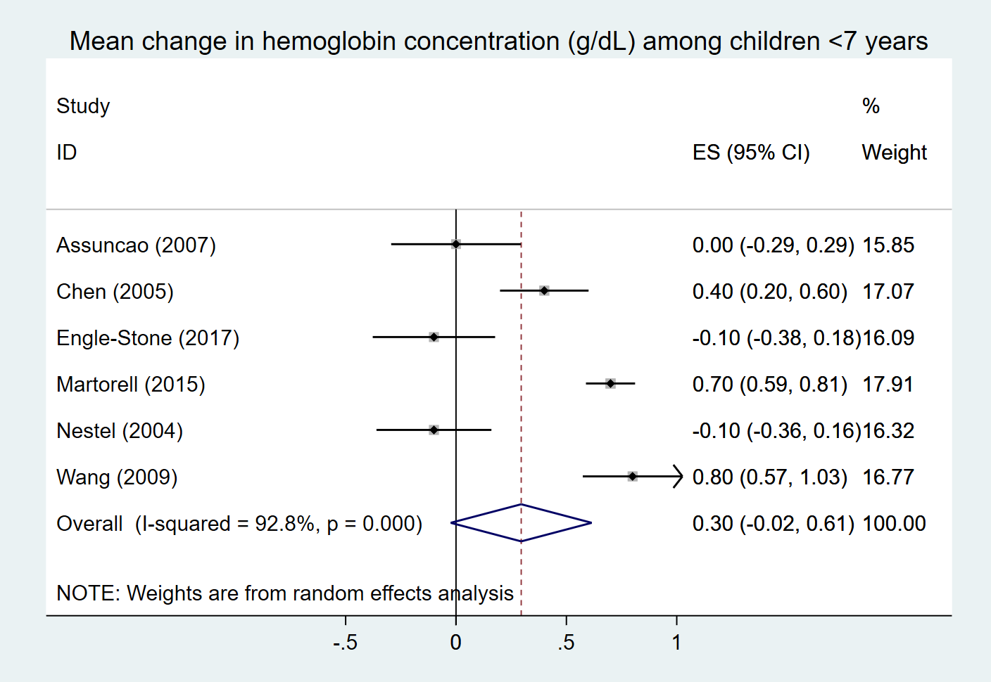
In forest plots, each study included in the meta-analysis is typically given a row in the plot and the effect size from that study will be marked as a square at the appropriate point on the X-axis. The size of the square represents the weight given to that study in the meta-analysis and the bars coming out of the square represent the uncertainty interval of the effect size from that specific study. The effect sizes and weights of each study are generally listed on the forest plot as well (see the right side of the plot above). The diamond at the bottom of the forrest plot represents the summary effect size with the top and bottom vertices of the diamond placed on effect size value on the x-axis and the left and right vertices of the diamond placed at the uncertainty ranges for the effect size.
Note
The forest plot shown above uses random effects analysis and the included studies are all given relatively similar weights, so the boxes for each study are very similar in size.
If fized effects analysis were to be used, there would be more variation in the weights and box sizes for each study.
Publication Bias - Funnel Plots
An important consideration when conducting meta-analyses is the possibility of publication bias. Publication bias occurs when the outcome of a research study or trial influences the decision to publish. For instance, researchers who find a significant association between a treatment and outcome may be more likely to publish their findings than researchers who find no association between a treatment and outcome because it may be interpreted as a “non-finding.” Further, if researchers find a result that was the opposite of the expected finding, they may choose not to publish the results due to the perception that the results may not be valid.
Publication bias can lead to bias in using meta-analysis to estimate a summary effect. Consider the following scenario:
Let’s say that there is interest in the news about whether eating fruit is associated with clinical depression. Let’s also say that there are 30 nutritional epidemiologists who have large datasets available on nutritional habits and mental health who see this news and think, “wow, I should investigate this association in my data.” Ten of the epidemiologists find a positive association between fruit and clinical depression and think, “wow, I should publish these results!” and do. Another ten of the epidemiologists find no association and the remaining ten find a negative association and think, “huh, must have been nothing to those news stories” and do not publish thier findings.
Then, another researcher notices that several studies have reported an association between fruit consumption and clinical depression and decides to perform a meta-analysis on the available studies. That researcher collects the 10 published studies and finds that there is a significant positive association! However, if all 30 of the studies conducted had been published and available for inclusion in the meta-analysis, the researcher would have likely found no association!
One way to assess for the presence of publication bias is to make a funnel plot. The x-axis of a funnel plot is effect size and the y-axis is the confidence in the effect size (standard error, plotted from high to low). Each study eligible for inclusion in a meta-analysis is then plotted on these axes.
If no publication bias is present, the points on the plot should be arranged in a pyramid (or inverted funnel) shape such that the studies with the most precision (high on the y-axis) will fall close to the center of the pyramid (average effect size) and studies with lower precision (lower on the y-axis) may fall farther from the center of the pyramid, with equal distribution on either side*.
If the points on a funnel plot show significant asymmetry, it is likely that publication bias may be present.
Notably, funnel plots are a rather crude assessment of publications bias and may also represent other potential biases in the studies (ex: small studies may be more subject to selection bias that may result in systematic under- or over-estimation of the effect size).
Todo
Include exmaple funnel plot